Forecast Weather Models

**Figure 1** An example of model output across the continental United States. This example contains information from the Global Forecast System (GFS) model, run by the National Weather Service.

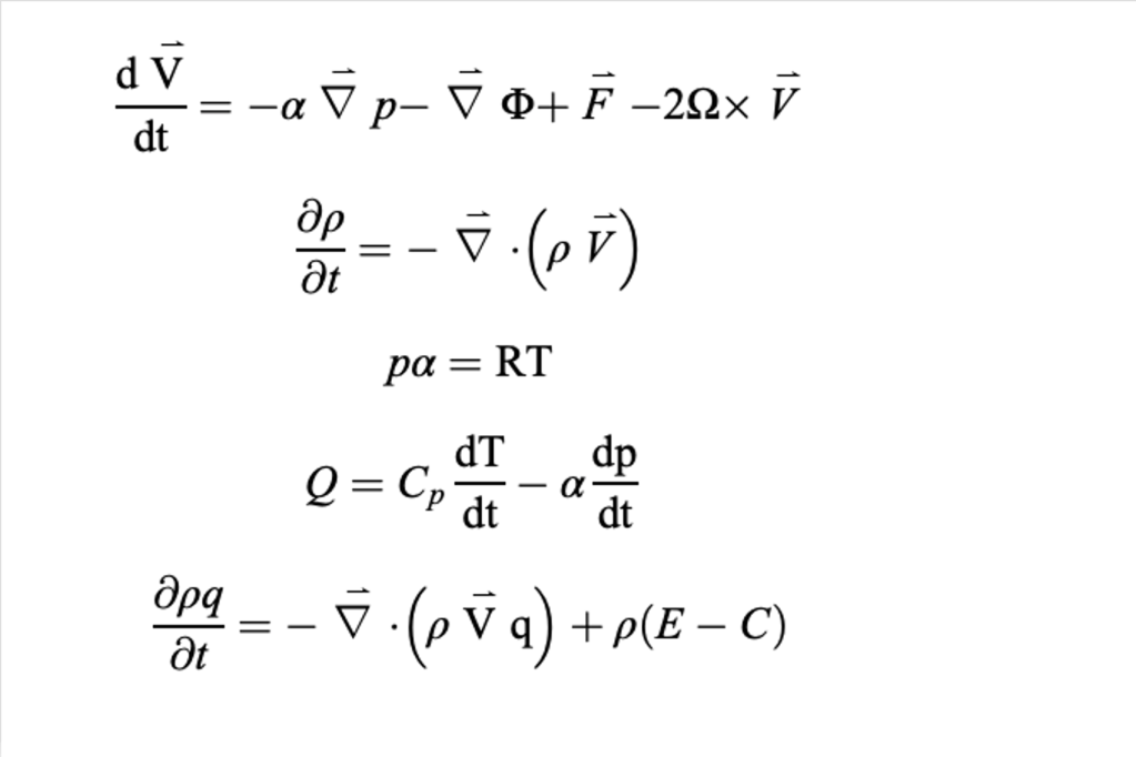
At their simplest, weather forecast models are a collection of programs that collect data, ensure it fits a prescribed format, then feeds the data into a program that solves equations that govern the how air moves through the atmosphere. At their most complex, weather forecast models contain many modules that perform the above tasks on scales as large as the planet, and as small as a US state or two. At their core, weather forecast models solve the equations across the size of their domain (size of the map over which they are working) across three dimensions and time steps until they reach the end of the predetermined time for the forecast to end.

Because of the awesome task laid out before them, weather forecasts models are some of the most complex software packages ever authored, and until not all that long ago, demanded the fastest computers on the planet to complete their critical tasks in the shortest period possible. While many of the details of how computer models work lie beyond the scope of this journal, we will endeavor to cover many of the most crucial topics so that you can gain at least a rudimentary understanding of what forecast weather models do, how they work, and what they do well (and perhaps not so well).

A Brief History of Numerical Weather Forecasting

**Figure 2** These are the equations of motion that govern the motion of air in the atmosphere. These equations are exceedingly complex (inducing nightmares in meteorology students) and require the fastest computers in the world to solve.

Though people have been observing weather since there have been people to observe weather, attempts to forecast weather started with the US Army Signal Corps in the 1860s, as higher speed communications allowed people to share current weather conditions more readily. It had been known for some time there existed a set of mathematical equations that could theoretically make forecasting much more accurate, but the lack of computing power left these dreams beyond the fingers of even the most optimistic weather forecasters.

Numerical weather prediction (NWP) uses mathematical models of the atmosphere and oceans to predict future states of both based on current conditions. The first rudimentary attempts to use these equations to forecast the weather were made in the 1920s, but it was not until the 1950s that computing power made these types of forecasts plausible. However, daunting roadblocks stood in the way of numerical weather prediction, as it was determined that the atmosphere was much more complex than originally believed.

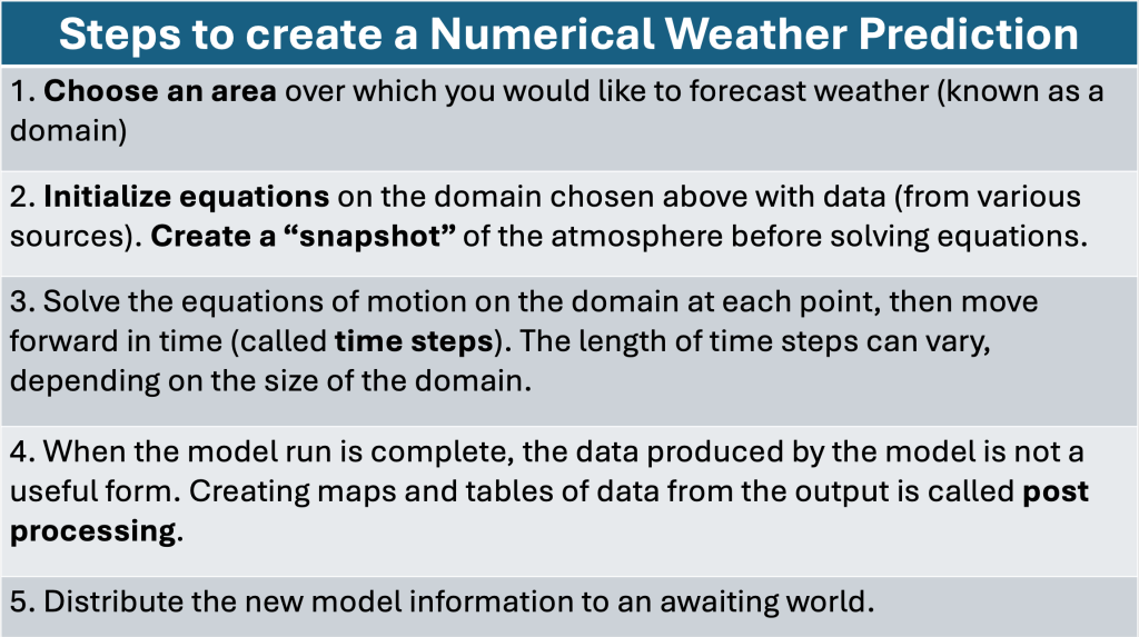
Building a Numerical Weather Prediction System

Once the equations of motion are programmed into the computer, the next step in creating a numerical weather forecast is creating the initial conditions of the atmosphere. In order to ensure that the equations have sufficient input, all of the weather data available in the atmosphere at a given time is made available (such as 1200 UTC, Universal Coordinated Time, a time frame used by scientists to make data is related in time). Many types of data are available for use in creating the initial conditions, such as data from weather balloons, aircraft data, information derived from weather satellites, as well as surface data and information from weather radar. Since the data comes from such disparate sources, it needs to be placed onto a grid that can be ingested into the set of equations (which we will refer to as forecast model moving forward).

Though numerical weather prediction has made incredible progress over the past few decades, making sure that data that is used as the initialization of the forecast model remains a problem for meteorologists. For many parts of the globe, there are large holes in the initialization process, meaning that the forecast model is not getting the best input it can to execute effectively. Other techniques (again beyond the scope of this blog entry) can aid in filling in the blanks, but having an incomplete set of data to feed into the forecast model remains one of the trickiest numerical weather prediction problems that remains. Errors introduced into this portion of the forecast process can be compounded with time, effectively limiting how far into the future computer models are accurately forecast.

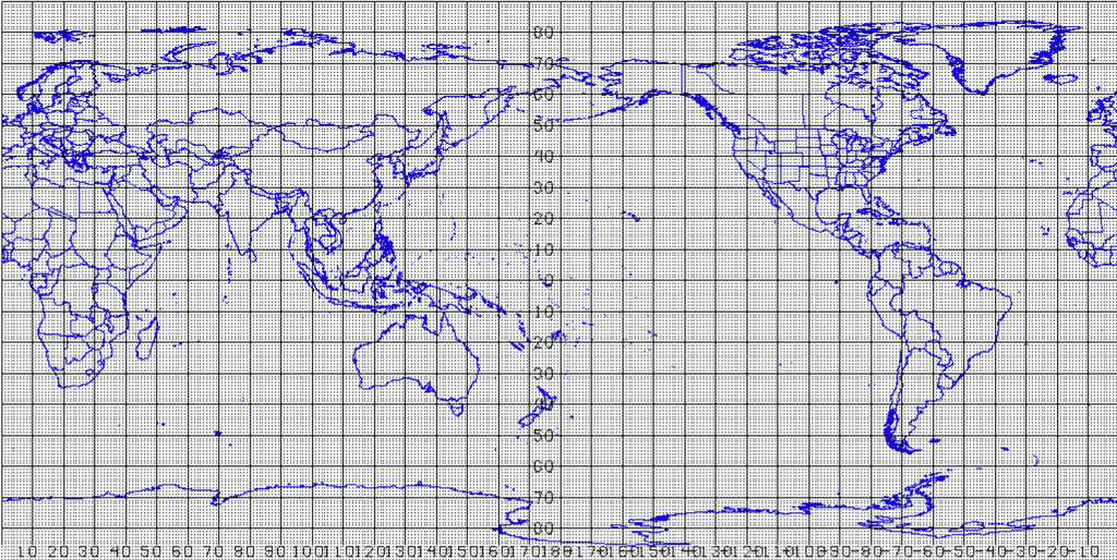
**Figure 3** The forecast domain for the model. The equations of motion are solved at each of these points across the two dimensional grid, as well as in the third dimension (which size is model dependent).

Once the initial data is placed on the forecast domain (the area over which you want to forecast, as seen in Figure 3), each of the equations of motion need to be solved for each point on the forecast domain, as well as in the third dimension (which depends on the model used). As you can see in Figure 3, the number of points at which these equations must be solved is daunting, and that is the primary reason that for many years the fastest computers in the world were used to forecast the weather.

After the equations are solved for all of the points shown above, the model is advanced forward a certain amount of time, before the equations are again solved with the information from the previous step. Known as a time step, the program is moved ahead by a few minutes before the equations are again solved. For larger models (which forecast for the entire globe), this number could be tens of minutes, and for smaller models, it may be as little as a couple of minutes. This process continues until all of the equations are solved for the amount of time of the forecast (for five days, for example).

**Figure 4** Supercomputers, like the ones located in Suitland, MD, are used to forecast the weather all over the globe.

Once the equations have been solved, the computer programs finish. The output created by the programs looks nothing like you might expect. Instead of detailed maps with important information outlined, the data is instead files full of data, waiting to be processed into something useful. Early forecast weather models were not nearly as sophisticated as today, and had difficulty properly adjusting the amount of heat and moisture in the atmosphere properly. When this occurred, low pressure systems were much too strong when created, producing too much rain and wind in one place, and not nearly enough in others. These errors made the model output useless, and required some ingenuity to remove them from the output. In order to adjust the raw model output, smaller programs adjusted the amount of heat and moisture during each step of the model run, attempting to prevent unrealistic output in the first place. Modelers using adjustment to prevent raw model data from becoming useless added parameters to the solutions, preventing the errors from growing too big, in a process called parameterization. Having to add these checks for each step in the model does cost time, but improves the output greatly.

The next step, known as post processing, takes the raw files and creates maps and tables of data that forecasters can recognize and use to forecast the weather. Depending on the amount of post processing needed, the process could take a few minutes, and when completed, the data is sent to a waiting world. During the early years of numerical weather prediction, the model output was sent via fax to land sites as well as ships as sea, and I used such maps during my college years as well as the beginning of my NWS career.

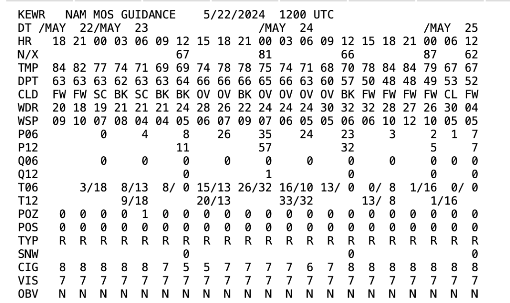
**Figure 5** A modern fax chart of winds and waves created by NOAA’s Ocean Prediction Center. Weather maps were routinely issued in this manner early in the numerical weather forecast process

During this process, model output statistics (MOS) are created, an attempt to balance some of the error introduced during the initialization process, as well as others errors. These statistics were created to correlate what the models do fairly well (like forecast the position of surface high and low positions) to what they do not do as well (such as forecast low temperatures in a valley on a cold, clear night). Additionally, using these relationships, the chance of precipitation can be computed. Models show where rain is expected, but does not account for errors in the model itself; MOS products can.

**Table 1** MOS for Newark, NJ (KEWR). Coded messages hold a tremendous amount of information used by forecasters for differing tasks on a daily basis.

**Table 2** A review of the steps necessary to run a forecast weather model and produce output.

One Forecast, Many Ways of Getting There

Please be aware: These steps cover the very basics about how forecast models create information for forecasting the weather. Since there are sources of error introduced throughout the process, different entities wishing to produce weather forecasts use different approaches when it comes to how to initialize data, choosing the size of the domain and how far our in time to run the model. Because of these differences, there are many applications of numerical weather prediction when it comes to forecasting the weather.

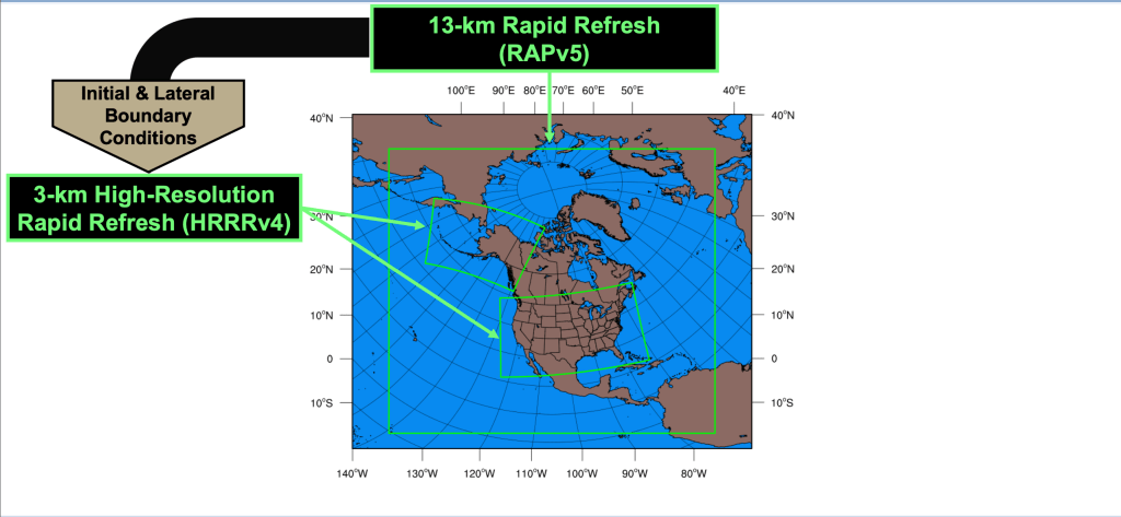
Most forecast weather models are run by government entities or universities testing new ways of initializing data or different ways to show the data (known as data visualization). In the United States, the National Weather Service runs models as large as the Global Forecast System (GFS), which forecasts weather for the entire globe, the North American Model (NAM), which forecasts for mainly North America, and much smaller models such as the High Resolution Rapid Refresh (HRRR), which runs hourly over a subset of North America. Each of these models excels during portions of the forecast process, while others are used to fine tune the solutions of the larger model forecasts.

**Figure 6** Image showing over which areas the HRRR model is run. Since it runs once an hour, it forecasts over a much smaller area than the GFS (seen in Figure 2).

In addition, many countries throughout the world run their own forecast models, with emphasis put on the forecast challenges their areas present. However, the non-US model discussed most across the globe is the European Centre for Medium Range Forecasting (ECMWF). Created by a for-profit conglomeration located in England, this model drew international interest when it successfully forecast the position of SuperStorm Sandy along the NJ coast at the end of October 2012 much earlier than other models. This model runs on some of the fastest computers in the world, and its designers employee unique approaches to initializing the data for the model (often cited as the most difficult portion of the numerical weather prediction process). The ECMWF is used to forecast for more than half of the globe, and forecasters in the US evaluate its output in making forecast decisions as well.

Ensemble Forecasting

Because of the differences in the way governments and universities approach numerical weather prediction, there are many forecast weather models available to meteorologists across the world. Most of the differences between models lie in how they initialize their solutions, and how they modify known problems (such as the distribution of moisture and heat, known as parameterization). Since there is no “perfect” initialization available. forecast model makers have been attempting to adjust for the errors introduced in this part of the process.

Modifying how models initialize their forecast runs can give forecasters some insight into how much of the error in the model solution produced is due to the initialization. Without wading too deeply into the math used, model builders vary the data in an initialization to match the error they have seen in previous forecast model runs. By perturbing (meaning to change by move in one direction or another) the initialization to mimic the errors seen in the past, and run models with these perturbations, we can determine how much the final model solutions are dependent on how they start.

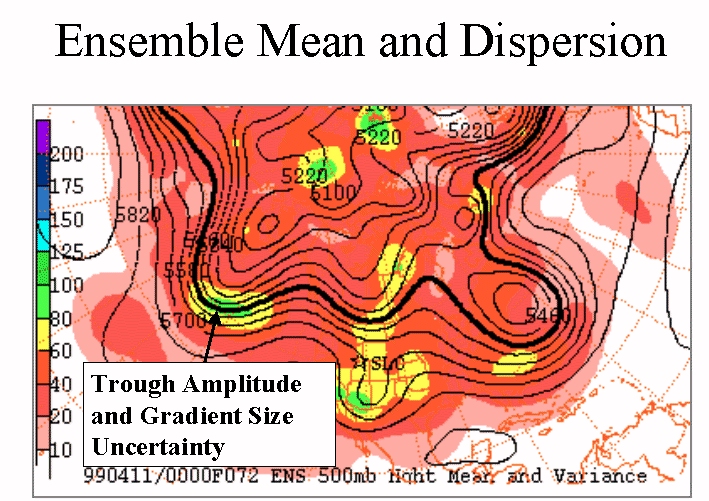
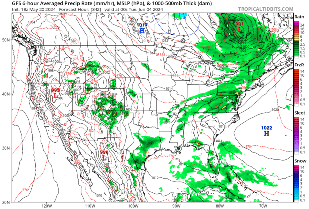
**Figure 7** Mid level (around 18,000 feet) forecast for the US. Places where the colors trend from yellow to green indicate where there is uncertainty in initial conditions. Running many forecasts with small changes in these areas could offer forecasts insight as to how much these changes matter in the forecast.

Perturbing the initial conditions where the colors transition from yellow to green would allow forecasters to determine to what extent these differences matter to the final forecast. It is beyond the scope of this journal entry (and honestly my math skills) to easily describe how these perturbations would be implemented, but running the model with each perturbation (as well as the original forecast, with no perturbations) would show how much spread (difference) in the forecast models there is by the end of the model run.

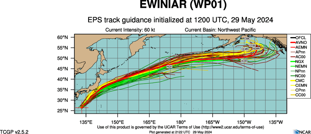
**Figure 8** UCARS ensemble information for a tropical system in the western Pacific.

If the differences between model runs is small, it can be deduced that the initial conditions were not as sensitive as suspected. Figure 8 shows an ensemble forecast for a tropical system in the western Pacific. Note that the tracks are quite similar, suggesting that initial conditions did not have a large impact on how the models are handling the system, lending confidence to the overall forecast. Greater “spread” (difference in the storm track) would indicate that the system is sensitive to initial conditions, lowering forecaster confidence in the system (for now).

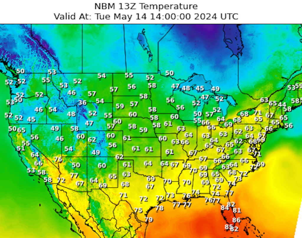
The National Blend of Models (NBM)

The National Blend of Models (NBM) is a nationally consistent suite of calibrated models based on the blend of NWS and other numerical weather models that produced post processed model guidance. The original goal of the NBM project was to create a highly accurate consistent starting point for use by NWS forecasters across the US.

National Weather Service forecasters have been largely editing gridded data forecasts to produce the text and images used every day since 2003. One of the main problems using this approach was assuring that there was no discernible “line” between forecast areas, making the maps appear as though they were created by one forecaster. Using the NBM greatly reduces this problem while offering forecasters a consistent starting point, making changes only where needed.

**Figure 10** An example of an NBM temperature for the continental US.

The NBM is indeed an ensemble forecast, though not exactly in the way we have seen. By using many different models (which have differing methods for dealing with model initialization and how to overcome other model deficiencies) that are calibrated for past performance helps overcome the differences and produce a multi model forecast solution.

Review

How computer models are built, run and used as tools by forecasters to identifying significant and routine weather has been reviewed here. Numerical weather prediction has been part of the forecast process since the 1950s, but increases in our understanding of how to model the atmosphere more accurately and sharp increases in computer power has had made the process much more reliable.

The process has become streamlined. with the basic steps outlined in the table above. Concepts such as ensemble forecasting were borne out of the continued research into numerical weather prediction, when it was discovered that how we feed data into the model has an impact on its performance. Ensemble forecasting has had a huge impact not only on forecasting but the way we convey uncertainty with respect to that forecast.

If this read was difficult, you have my apologies. If it is any comfort, I am not convinced that at least some operational forecasters have a much better understanding of the process. If you have any questions, please drop me a line.